Wednesday, 5 September 2012

CFA Level I: Quantitative Methods - Statistical Concepts and Market Returns (Part 1)

For other CFA Level I topics, click here

This topic is rather long, so I decided to split it into 2 parts. This part will cover the following items:
  • statistics concepts
  • frequency distribution
  • measures on central tendency (mean, median, mode)

1. Concepts:

Descriptive Statistics are used to summarized important characteristics of large data sets.
Inferential Statistics are tools used to draw larger generalizations from observing a smaller portion of data.

A Population is the set of all possible members of a stated group  
A Sample is a subset of the population of interest

Parameter is the measure used to describe a characteristic of a population.
Sample Statistics is used to measure a characteristic of a sample.
 
Types of measurement scales 
Level of measurement increases as we move down this list.
Nominal - observations are classified or counted with no particular order. Example: in a living room, number 1 is a table, 2 is a TV, 3 is a vase, etc.
Ordinal -  data is categorized according to some rank that helps to describe differences between data. Example: an IQ of 120 ranks higher than an IQ of 100. However, you can't say that the difference between IQs of 140 and 120 is the same as the difference between IQs of 120 and 100.
Interval - like Ordinal scale, this provide relative ranking but the difference between scale values are equal. Example: the difference between 30 and 20 degrees Celsius is the same as the difference between 60 and 50 degree Celsius. However, the weakness of this scale is that a 0 degree Celsius does not mean that there is no temperature. This means that interval-scale-ratios are meaningless.
Ratio - this scale provide ranking, equal difference, and a true zero point. Example: if you have $100, it means that you have 4 times as much as $25; and $0 means that you have no money.


2. Frequency Distribution:

Steps to construct a frequency distribution:

Step 1: Define intervals. Intervals must have lower and upper limits and are mutually exclusive (i.e. 1 observation can only fall to 1 interval). The total set of intervals should cover the total range of values for the entire population.
Step 2: Count the observations to get the Absolute Frequency (i.e. number of observations that fall within a given interval)

Other ways to present data

Relative frequency is calculated by dividing the absolute frequency of each interval by the total number of observations.
Cumulative Absolute Frequency and Cumulative Relative Frequency is the sum of absolute or relative frequencies starting at the lowest and moving up to the highest.

The following examples are taken from Kaplan SchweserNotes 2011 to illustrate the concepts.

The table below represents the returns on Intelco's stock
Annual Returns for Intelco Stock
10.4%
22.5%
11.1%
–12.4%
9.8%
17%
2.8%
8.4%
34.6%
228.6%
0.6%
5.0%
–17.6%
5.6%
8.9%
40.4%
–1.0%
–4.2%
–5.2%
21.0%

To construct Frequency Distribution for the data above:
Step 1: Define Interval.
The range of return = 69% = 40.4% – (–28.6%). We can use 8 nonoverlapping intervals of 10%
Step 2:
Interval
Absolute
Frequency
Relative Frequency
Cumulative Absolute Frequency
Cumulative Relative Frequency
–30% ≤ Rt < –20%
1
1/20 = 5%
1
5%
–20% ≤ Rt < –10%
2
2/20 = 10%
3
15%
–10% ≤ Rt < 0%
3
3/20 = 15%
6
30%
0% ≤ Rt < 10%
7
7/20 = 35%
13
65%
10% ≤ Rt < 20%
3
3/20 = 15%
16
80%
20% ≤ Rt < 30%
2
2/20 = 10%
18
90%
30% ≤ Rt < 40%
1
1/20 = 5%
19
95%
40% ≤ Rt < 50%
1
1/20 = 5%
20
100%
Total
20
100%


The interval with greatest absolute frequency is the 0% ≤ Rt < 10% interval. It is called the Modal Interval.

Histogram and Frequency Polygon are the graphical presentations of the absolute frequency distribution (see picture below)


3. Measures on Central Tendency

Population Mean is calculated is follows


Sample Mean is used to make inferences about the population mean
The population and sample mean are both arithmetic means, which is the sum of observation values divided by the number of observations.

The sum of the deviations from the mean is zero

Weighted mean takes into account the weights of different observations and is computed as follows:
Example: An investor has a portfolio with 35% stocks, 30% bonds, 20% cash, and 15% commodity. Their returns are 15%, 7%, 4%, and 8% respectively. What is the portfolio return?

Portfolio return = weighted mean of the returns = (0.35 x 0.15) + (0.3 x 0.07) + (0.2 x 0.04) + (0.15 x 0.08) = 0.0935, or 9.35%

The return of a portfolio is the weighted average of the returns of the individual assets in the portfolio. 

Median is the midpoint of a data set when the data is arranged in ascending or descending order. 50% of the observations are above and 50% are below the median. Median is a better measure of central tendency than arithmetic mean when there are extremely large or small values in the observations.

Example: Find medians of the following sets of data
a. 5, 12, 3, 9, 37
b. 4, 7, 2, 9, 16, 11

a. Arrange the numbers in descending order: 37, 12, 9, 5, 3. Median is 9 because it is the midpoint of the data set.
b. Arrange: 16, 11, 9, 7, 4, 2. With an even number of observations, the median is the arithmetic mean of the 2 middle observations, 9 and 7. Thus, median = (9 + 7)/2 = 8

Mode is the value that occurs most frequently in a data set. A data set may have more than one Mode or no Mode. 
A distribution is Unimodal when it has one value that appears most frequently .
When a set of data has 2 or 3 values that occur most frequently, it is said to be bimodal or trimodal. 


Geometric mean is computed as follows:
When calculating the geometric mean for a returns data set, it is necessary to add 1 to each value under the radical then subtract 1 from the result as follows:

Example: the returns of a stock over 4 years are 10%, –20%, 5%, and –4% respectively. Compound the annual rate of return over the 4-year period.

1 + RG = [(1 + 0.1)(1 – 0.2)(1 + 0.05)(1 – 0.04)]1/4 = 0.9705
RG = –0.0295 = –2.95%

Harmonic mean is used for calculations such as average cost of shares purchased over time.

Example: an investor purchase $1000 stock each month, and over the past 3 months prices per share were $8, 10$, $5. Calculate the average cost per share.

average cost per share = harmonic mean = 3/(1/8+1/10+1/5) = $7.06

Monday, 3 September 2012

CFA level I - Quantitative Methods: Discounted Cash FLow Applications

For other CFA level I topics, click here 

1. Net Present Value (NPV) & Internal Rate of Return (IRR)

Net present value (NPV) is the difference between the present value of cash inflows and the present value of cash outflows of an investment.

To solve a NPV problem, you just need to find the present value of all the cash flows from the investment. The sum of all these present values is the Net present value of the investment

Example: Calculate the NPV of an investment project with initial cost of $4 million and clash flows for the next 5 years as follows:
year 1: $900,000
year 2: $1.2 million
year 3: -$500,000
year 4: $700,000
year 5: $2 million
Given the discount rate of the project is 11%

NPV = -4 + 0.9/1.11 + 1.2/1.112 + (–0.5)/1.113 + 0.7/1.114 + 2/1.115 = –$0.9328 million = –$932,800 
This project has a negative Net Present Value

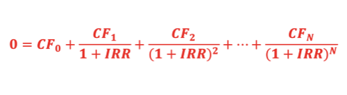
Internal Rate of Return (IRR) is the rate of return that makes the net present value of all cash flows from a particular project equal to zero. In other words, it makes PV of inflows = PV of outflows.
Usually CF0 represents the initial cash flow/cost of an investment and is therefore negative. Solving for IRR is most of the time through trial error.
Let r be the required rate of return of an investment, if:
  • r < IRR gives NPV > 0
  • r > IRR gives NPV < 0 

NPV Decision Rule
  • Accept the project with NPV > 0
  • Reject the project with NPV < 0
  • When only 1 of the projects can be accepted, choose the project with higher positive NPV 

IRR Decision Rule
  • Accept projects with IRR > r (investors' required rate of return)
  • Reject projects with IRR < r 

*** When NPV and IRR rules give conflicting decisions, always go for the project with the greatest NPV 


2. Holding Period Return, Money-weighted and Time-weighted rates of return

Holding Period Return (HPR) is the percentage change in the value of an investment over the period it is held. If the assets have cash flows such as dividends, the return, including these cash flows, is called Total Return.

HPR = (P1 – P0 + D1)/P0


          P0 = the initial investment
          P1 = price received at the end of the holding period
          D1 = cash paid by the investment by the end of the holding period
 

Example:
a. A share of stock is purchased at $50 & sold for $60 six months later. Calculate HPR.
b. Consider the same stock, this time, during the 6-month period, it paid $2 in dividends.


a. HPR = (60 – 50)/50 = 20%
b. HPR =  (60 – 50 + 2)/50 = 24%


Money-weighted Rate of Return is another name for the Internal Rate of Return (IRR). To solve the Money-weighted rate of Return problem, solve the following equation:

PV (outflows) = PV (inflows)

Example: Consider an investment that cover a duration of 2 years. At time t = 0, an investor bought 1 share at $200. At time t = 1 he bought another share at $225. At the end of the second year (t = 2), he sold both shares for $235 each. During both years, the stocks paid per-share dividends at $5. the dividends are not reinvested

We first need to identify cash outflows and inflows
Outflows: 
at t = 0, $200 to purchase the first share
at t = 1, $225 to purchase the second share
Inflows:
at t = 1, $5 dividend from the first share
at t = 2, $10 dividend from the 2 shares
at t = 2, $470 from selling both shares

Let r be the money-weighted rate of return
PV (outflows) = PV (inflows)
200 + 225/(1+r) = 5/(1+r) + (470+10)/(1+r)2
Through trial and error, we get r = 9.39%


Time-weighted Rate of Return measures compound growth . It is the rate at which $1 compounds over a specified performance horizon. To solve for the annual time-weighted return, follow these steps:
  • Step 1: Price the portfolio immediately prior to any significant addition or withdrawal of funds. Form subperiods based on the cash inflows and outflows.
  • Step 2: Calculate the HPR on the porfolio for each sub period.
  • Step 3: Compute the product of (1+HPR) for each subperiod to get total return for the entire measurement period
    i.e., (1+
    HPR1) x (1+HPR2) x ... x (1+HPRN)
    If the total investment period is greater than 1 year, you must take geometric mean of the measurement period return to find the annual time-weighted rate of return

Example: an investor purchased a share of stock at t = 0 for $100, at the end of next year t = 1, he bought another for $120. At the end of t = 2, both shares are sold for $130 each. Dividend for each of the stock in year 1 and 2 is $2 per share. Solve for the annual time-weighted rate of return for this investment.


Step 1: Break the evaluation period (2 years) into subperiods based on timing of chas flows:
Holding Period 1
    Beginning value = $100
    Dividends paid = $2
    Ending value = $120 (this is the value of the first share at after 1 year)
Holding Period 2
    Beginning value = $240 (2 shares, $120 each)
    Dividends paid = $4 ($2 per share)
    Ending value = $260 (2 shares)

Step 2: Calculate HPR for each period
HPR1 = [(120 + 2)/100] – 1 = 22%
HPR2 = [(260 + 4)/240] – 1 = 10%

Step 3: Find the compound annual rate that would have produce a total return equal to the return on the investment over 2-year period
(1 + time-weighted rate of return)2 = (1.22)(1.10)
Since the investment period is 2 years long, we have take geometric mean of the result above to get the time-weighted rate of return.
[(1.22)(1.10)]0.5 – 1 = 15.84%


3. Bank Discount Yield (BDY), Holding Period Yield (HPY), Effective Annual Yield (EAY), and Money Market Yield


T-bills are quoted on bank discount basis, which is based on the face value of the instrument instead of the purchase price. The Bank Discount Yield (BDY) is computed as follows: 

Note that a yield quoted on a bank discount basis is not representative of the return earned by an investor.

Example: calculate BDY for a T-bill priced at $96,500, with a par value of $100,000 and 120 days until maturity

rBD = 3,500/100,000 x 360/120 = 10.5% 

Holding Period Yield (HPY) is the total return an investor earns between the purchase date and the sale or maturity date.  Formula for Holding Period Yield is exactly the same as Holding Period Return (HPR) in section 2.

HPY = (P1 – P0 + D1)/P0


          P0 = the initial investment
          P1 = price received at the end of the holding period
          D1 = cash paid by the investment by the end of the holding period


Effective Annual Yield (EAY) is an annualized value, based on 365-day year, that accounts for compound interest

                              EAY = (1 + HPY)365/t – 1


Example: Calculate EAY for a T-bill priced at $96,500, with a par value of $100,000 and 120 days until maturity.

HPY =  (100,000 – 96,500)/96,500 = 3.6269%
EAY = (1.036269)365/120 – 1 = 11.45%

Money Market Yield (or CD Equivalent yield) = annualized HPY, assuming 360-day year
Bond Equivalent Yield refers to the 2 x semiannual discount rate. This stems from the fact that yields on US bonds are quoted as twice the semiannual rate because coupon is paid in 2 semiannual payments

Example 1: a 3-month HPY of 2%. Find yield on bond-equivalent basis.

Step 1: convert 3-month yield to effective semiannual yield:  1.022 – 1 = 4.04%
Step 2: double it to get the bond-equivalent yield 2 x 4.04 = 8.08%

Example 2: If effective annual yield on an investment is 8%. to calculate the bond-equivalent yield:

Step 1: Convert effective annual yield to effective semiannual yield:   1.080.5 – 1 = 3.923%
Step 2: double it 2 x 3.923 = 7.846%